Contrast curves
Creation of a DetectionMap instance
In addition to the characterization of stars and substellar objects, MADYS provides another particularly useful feature for the high-contrast imaging (HCI) community: namely, the capability to convert detection limit curves of a HCI observation into mass limit curves and completeness maps.
The computation is mediated by the DetectionMap class. Let us analyze the syntax needed to initialize an instance:
file = "examples/SPHERE_contrast_curve.fits"

params = {'parallax': 5.8219, 'parallax_error':0.31,
          'ebv': 0.04, 'ebv_error': 0.01,
          'app_mag': 6.182, 'app_mag_error': 0.233,
          'band': 'SPH_K1', 'age': 16.,
          'age_error': 7.
         }

curve = DetectionMap(file, 'contrast_map', params)
The basic inputs needed to create an instance are therefore:
file: path-like, numpy array or tuple, required. Input contrast curve. It can be:if
file_type= ‘contrast_separation’:a 2D numpy array, with size (n_points, 2), where the first column stores contrasts, the second one separations in arcsec;
a tuple (contrasts, separations), with the two items being numpy arrays as in 1);
a valid .fits file containing the data, formatted as in the array case. In this case, two keywords
OBJECTandPIXTOARCare expected in the header, corresponding to the name of the star and the platescale in mas/px.
if
file_type= ‘contrast_map’:a 2D numpy array, with size (n_x, n_y), representing the contrasts achieved for any pixel in the original image;
a valid .fits file containing the data, formatted as in the array case.
file_type: string, required. It can be either:‘contrast_separation’, if a 1D curve(separation) with shape (n_points, 2) is provided;
‘contrast_map’, if a 2D curve(x, y) is provided. A 3D map (lambda, x, y) is accepted too.
stellar_parameters: dict, required. A dictionary containing information for the star under consideration. The following keywords must be present:‘parallax’: float. Stellar parallax [mas];
‘parallax_error’: float. Uncertainty on stellar parallax [mas];
‘app_mag’: float. Apparent magnitude of the star in the ‘band’ band [mag];
‘app_mag_error’: float. Uncertainty on ‘app_mag’ [mag];
‘band’: string or list. Filter(s) which the map refers to. It (They) should be valid filter name(s) for MADYS. If the input map is a 3D map (band, x, y), a list can be used to attribute the individual slices along the first axis to different bands. In this case, the program will convert each slice individually and then take (pixel-wise) the best mass limits.
‘age’: float. Stellar age [Myr];
one between:
‘age_error’: float. Uncertainty on stellar age [Myr]. It must be larger than 0.
a couple ‘age_min’, ‘age_max’: float. Lower and upper values for stellar age [Myr]. ‘age’, ‘age_min’, ‘age_max’ must strictly satisfy the relation: age_min < age < age_max.
For extinction, two possibility exist:
either it is set explicitly through the following doublet of keywords:
‘ebv’: float. E(B-V) reddening for the star [mag];
‘ebv_error’: float. Uncertainty on E(B-V) [mag];
or coordinates must be specified to allow the program to estimate E(B-V):
‘ra’: float. Right ascension of the star [deg];
‘dec’: float. Declination of the star [deg].
‘ext_map’: string, optional. 3D extinction map used for the computation. Possible values: ‘leike’, ‘stilism’. Default: ‘leike’. In this case, the error on ebv is always set to 0.
In addition to this, a dictionary is required to be supplied through the keyword sequence_parameters if file is not a path to provide missing information. Its keywords are:
‘OBJECT’: string. Name of the star;
‘PIXTOARC’: float. Platescale [mas/px] (only mandatory if file_type = ‘contrast_separation’).
Finally, an optional dictionary can be provided through the keyword exodmc_parameters. This specifies the parameters of the grid for all the completeness maps created from this instance.
Once created, the instance possesses the following attributes:
file: path-like, numpy array or tuple. Corresponding to input ‘file’.file_type: string. Corresponding to input ‘file_type’.stellar_parameters: dict. Corresponding to input ‘stellar_parameters’.data_unit: string. Corresponding to input ‘data_unit’.rescale_flux: float. Corresponding to input ‘rescale_flux’.minimum contrast: float. Corresponding to input ‘minimum_contrast’.contrasts: numpy array. Renormalized contrast curve (flux ratio).contrasts_mag: numpy array. Renormalized contrast curve (magnitude contrast).header: fits.Header(). Header of the input file (empty header if file is not a filepath).abs_phot: numpy array. Absolute magnitudes in the required filters.abs_phot_err: numpy array. Uncertainties on absolute magnitudes in the required filters.abs_phot: numpy array. Apparent magnitudes in the required filters.abs_phot_err: numpy array. Uncertainties on apparent magnitudes in the required filters.mag_limits: numpy array. Limit absolute magnitudes corresponding to input curve.mag_limits_err: numpy array. Uncertainties on limit absolute magnitudes.mag_limits_app: numpy array. Limit apparent magnitudes corresponding to input curve.mag_limits_app_err: numpy array. Uncertainties on limit apparent magnitudes.separations: numpy array. Input separations, if ‘file_type’=’contrast_separation’; zero-filled array otherwise.band: string. Input stellar_parameters[‘band’].platescale: float. Platescale of the instrument FOV [mas/px].object: string. Object name.exodmc_object: ExoDMC instance. It defines the grid of parameters across which DPM are evaluated.mass_limits: dict. It stores the mass_limits produced byDetectionMap.compute_mass_limits()to avoid repeating the computation if the model does not change.
Creation of mass curves
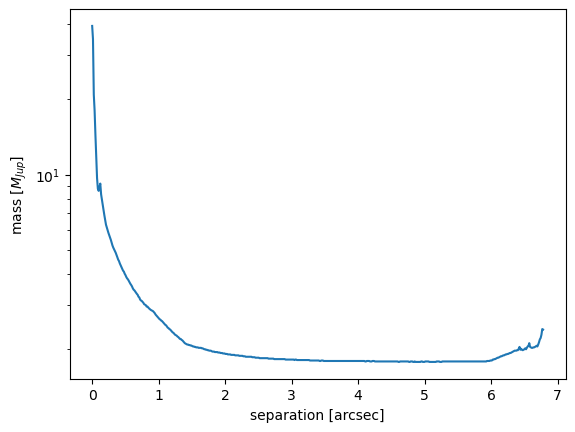
Starting from the object create above, it’s easy to compute the corresponding mass curve through the function DetectionMap.compute_mass_limits():
mass_limits = curve.compute_mass_limits('atmo2020-ceq')
If ``file_type``=’contrast_map’, the program will additionally collapse the map along the azimuthal direction, yielding a (N-1)-dimensional output in addition to the N-dimensional mass curve.
The output of DetectionMap.compute_mass_limits() is a dictionary, containing several outputs depending on the input type. In particular, the 1D mass curve – stored in the kwyrods map_1D – is a 3D numpy array where the first axis has three elements, corresponding to each of [age_opt, age_min, age_max]; the second axis represent the length of the two arrays; the third axis has two indices, one for the separation and one for the mass curve.
mass_array = mass_limits['map_1D'][0, :, 0]
separation_array = mass_limits['map_1D'][0, :, 1]

plt.plot(separation_array, mass_array)
plt.yscale('log')
plt.xlabel('separation [arcsec]')
plt.ylabel(r'mass [$M_{Jup}$]')
plt.show()
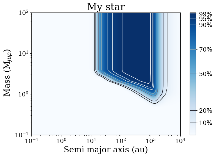
Detection probability maps: basics
A completeness map, or detection probability map, is a way to account for the observational biases underlying a direct imaging observation. Given a planet mass and a semi-major axis, it quantifies the probability that such a planet be detectable in the observation. This is particularly important in the context of surveys, where the true occurrence rate of planets must take into account the uneven coverage of the parameter space.
MADYS employs ExoDMC (Bonavita 2020) to create a grid of orbital parameters. For each planet mass and semi-major axis, 1000 orbits are randomly generated; after estimating the resulting projected separation, the planet’s flux (estimated from its mass and age) is compared to the contrast limit at that separation.
As mentioned above, the parameters of ExoDMC can be set using the keyword exodmc_parameters when the instance is initialized. The dictionary can have the following keywords:
x_min: float. Lower limit for grid x axis (default = 1);x_max: float. Upper limit for grid x axis (default = 1000)nx: int. Number of steps in the grid x axis (default = 100)xlog: bool. If True the x axis will be uniformly spaced in logy_min: float. Lower limit for grid y axis (default = 0.5)y_max: float. Upper limit for grid y axis (default = 75)ny: int. Number of steps in the grid y axis (default = 100)ylog: bool. If True the y axis will be uniformly spaced in logngen: float. Number of orbital elements sets to be generated for each point in the grid (default=1000).e_params: dict. Specifies the parameters needed to define the eccentricity distribution. If used, the following keys can/must be present:‘shape’: string, required. Desired eccentricity distribution. Can be uniform (‘uniform’) or Gaussian (‘gauss’)
‘mean’: float, optional. Only used if shape = ‘gauss’. Mean of the gaussian eccentricity distribution.
‘sigma’: float, optional. Only used if shape = ‘gauss’. Standard deviation of the gaussian eccentricity distribution.
‘min’: float, optional. Only used if shape = ‘uniform’. Lower eccentricity value to be considered.
‘max’: float, optional. Only used if shape = ‘uniform’. Upper eccentricity value to be considered.
Default: ‘shape’ = ‘gauss’, ‘mean’ = 0, ‘sigma’ = 0.3.
i_params: dict. Specifies the parameters needed to define the inclination distribution. If used, the following keys can/must be present:‘shape’: string, required. Desired inclination distribution. Can be uniform in cos(i) (‘cos_i’) or Gaussian (‘gauss’)
‘mean’: float, optional. Only used if shape = ‘gauss’. Mean of the gaussian inclination distribution [rad].
‘sigma’: float, optional. Only used if shape = ‘gauss’. Standard deviation of the gaussian inclination distribution [rad].
Default: ‘shape’ = ‘cos_i’.
Note
xlog and ylog are False by default in ExoDMC. However, we strongly advise the user to set xlog and ylog to True to avoid losing sensitivity at the low-mass and the low-sma edges, where the most interesting information is found.
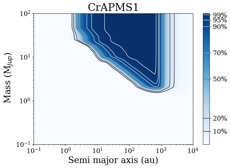
Let us create now a detection probability map:
Detection probability maps: advanced
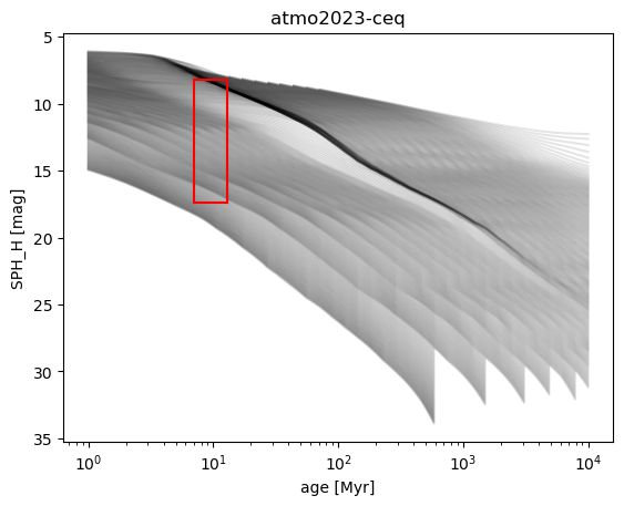
Sometimes, the dynamical range of a model are not sufficient to cover the entire age/mass range that is desirable. An example is provided in the image below:
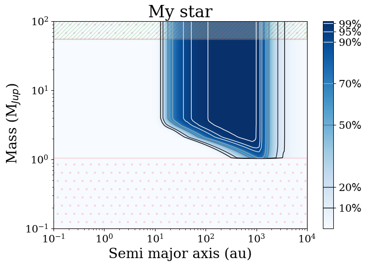
where the dotted area indicates the region where the model matrix is nan-filled. This can be seen explicitly by calling the helper function DetectionMap.visualize_grid_coverage():
In such cases, the user might consider activating the extrapolation option (see here for usage and caveats).